Processing of Helical Filaments

There is large overlap with generic single particle analysis (SPA) and some aspects are not covered in detail here (E.g., focal pair handling and CTF correction).

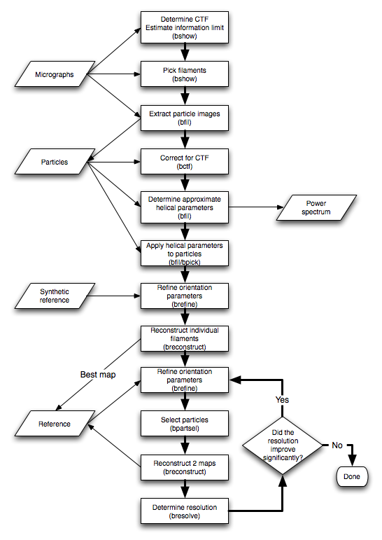
1. Preparation and initial processing

Helical processing occurs largely by single particle methods, and the typical directory organization is similar to that for SPA. The micrographs are set up and CTF determined in the same way as for SPA.

2. Filament picking

2.1. Picking filaments in bshow

Filaments can be picked in bshow using the filament tool. The filaments can be extracted for further inspection.

2.2 Converting filaments to particles

Filaments can be converted to overlapping particles, simply specifying parameters in bshow or with bfil. As with SPA, the user needs to decide on the size of particle box, considering that some sizes will process faster. The size must include a significant length of the filament, while not having too much bending across the box. In addition, the overlap between boxes along a filament must be chosen. The typical overlap ranges from 50 - 90% of the box size.

 

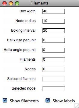
Prior to selecting the "Filament/Generate particles" menu option, the following parameters should be considered:

• Boxing interval: This determines the frequency of boxes along the filament and their overlap.
• Helix rise and angle per unit: The initial rough view for the particle is set based on the filament orientation and helical parameters. This can be used to reconstruct an initial map.

Once these parameters are set, the "Filament/Generate particles" menu option creates a set of boxes defining particles for extraction (see the particle picking tool).

2.3. Finding filament and particle locations in the closer-to-focus micrographs

Once all the filaments and particles have been picked in the further-from-focus micrographs, the closer-to-focus micrographs can be aligned to the further-from-focus micrographs as described for SPA (SPA mg alignment).

2.4. Particle extraction

Once all the particle coordinates are specified in the parameter files, the particle images can be extracted (change to the part directory first):

The -powerspectrum option generates an aligned power spectrum from all the selected particles. This can be used to inspect the layer lines and deduce helical parameters.

All the particle image files should be written to the part directory.

3. Initial reference

Specification of the helical parameters during particle generation or extraction presents the opportunity to reconstruct initial reference maps. To calculate one map per filament, use the -filaments option in breconstruct:

Each reconstruction can be examined for the best and used as a reference to determine orientations.

The key is to select approximately correct helical parameters, which means this approach will not work without a reasonable knowledge of these parameters.

The alternative is to synthesize a helical reference map, where the helical parmaeters should also be known to a reasonable extent.

4. Determining particle orientations

The filament particle orientations can be determined with borient or refined with brefine, using a suitable reference map. For each run of orientation-finding, create one directory such as run1, run2, etc.

4.1. Global orientation search

A grid search can be performed, taking into account that a filament lies approximately perpendicular to the electron beam, excluding a large part of the view unit sphere. The same program is used as for SPA, with the difference being specification of helical symmetry and the maximum angular deviation from a perfect side view (-side option):

4.2. Orientation refinement

Given already reasonable orientations for the particles, these parameters can be refined using a local search around the input views. There are two ways to do this. The first is using a Monte Carlo approach (i.e., adjusting parameters by small random amounts):

The second method does a 3x3x3 grid search around the input view starting at a given angular increment. If the maximum correlation coefficient is on an edge of the grid, a new grid is placed with this view in the middle and analyzed. If the maximum is in the center of the grid, the grid is contracted around it and analyzed. The grid is contracted until its angular increment falls below that of the second parameter, the accuracy:

5. Particle selection

The selection of particles for reconstruction is done as for SPA. In addition, the particles associated with one filament may not be all in a consistent direction. To fix the direction for each filament, use the -filament option in bpartsel during selection:

6. Reconstruction

The reconstruction can then be done from the selected particles. Typically, two reconstructions are generated from two different particle sets (option -multiple):

The resultant reconstructions have the inserts "_01" and "_02" before the extension and is used for resolution estimation (see next section). These maps can be added to generate a single reconstruction:

Reconstructions can also be done from a specific selection number in the parameter file using the "-select" option.

7. Resolution determination

The resolution determination is done as for SPA.

8. Determination of helical parameters

The helical parameters for the reconstruction can be refined by a search for the angular rotation that gives a maximum cross-correlation. This can be done in real space or reciprocal space, each with its own nuances that may make it work better than the other. The reciprocal space search only requires starting, ending and incremental values for the rotation angle:

This iterates through the angles from 50° to 70° in 0.5° increments and cross-correlates the original map with the map rotated around the z-axis and within the resolution limits. The helical rise is inferred from the offset of the cross-correlation peak and its absolute value should increase with increasing angle. This only works if the reconstruction already has the correct helical character.

The real space search is done on a grid of helical rise and rotation angle and requires starting, ending and incremental values for both the rise and rotation angle:

The map is rotated and shifted according to the helical parameters and the real space correlation with respect to the original map calculated within the radius specified.

9. Helical symmetrization

Once the parameters are known, helical symmetry can be imposed on the map:

This map is then used as a reference for subsequent particle orientation determinations.

Bernard Heymann 20121210