Single Particle Analysis - Resolution-limited version

Note that the following protocol assumes that focal pairs of micrographs were taken. In the event that only single micrographs were taken of each field-of-view, the step to align micrographs with bmgalign can be omitted.

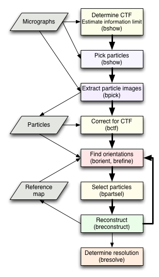
1. Preparation

SPA in Bsoft has been designed to fit nicely into a specific workflow and a specific directory organization. Within a particular project, a set of subdirectories at a single level should be created  to deal with the different stages of processing. Table 1 shows  the list of directories typically used.

Table 1: Suggested directories for SPA in Bsoft

Directory	Purpose
mg	Raw micrographs
mg_b2	Micrographs binned two-fold
part	Particle images extracted from the micrographs
ctf	CTF-corrected particle images
ref	Initial reference map(s) for orientation-finding
run1	First run of determining particle orientations with the resultant reconstruction(s)
run2	Second run of determining particle orientations with the resultant reconstruction(s)
...	...

Put all the micrographs in the mg directory.

All programs handling parameter files (i.e., STAR files) can read multiple files and concatenate them into one large internal parameter database. The whole internal database is then written out into one parameter file by specifying the "-output" option. If the user requires individual parameter files for each micrograph, the program bmg has a "-split" option to generate one parameter file per micrograph. Some of the programs also allow the user to set the path for files, which becomes very important to ensure a smooth and easy workflow.

2. Options to generate the first parameter files

The first micrograph parameter files can be generated in various ways as follows:

2.1. Generating parameter files from micrograph images:

The simplest is to use the micrographs themselves to write new parameter files:

This will generate the first parameter file with the micrographs arranged as pairs in each field-of-view (option -number) with the correct pixel size (option -Pixelsize), voltage (option -Volt), Cs (option Cs), amplitude contribution (option -Amplitude) and the appropriate paths for the micrographs (option -mgpath) and the particle images (option -partpath). The parameter file can be split into multiple files, each referencing just one micrograph:

Parameter files now have names corresponding to the original input micrograph files, and each can be opened in bshow to determine the CTF parameters.

2.2. Generating parameter files from bshow:

The second way is to open each micrograph individually in bshow, calculate the power spectrum, and fit the CTF parameters. After fitting the CTF, the parameters are written to a new parameter file.

2.3. Automated CTF fitting and generating parameter files:

The most advanced way is to run an automated CTF fitting first on each micrograph, generating a parameter file for each. The resultant fits need to be checked and refined in bshow. The micrographs can be processed one at a time:


Alternatively, a script can take care of the whole set (see the script prepfit).

In every case, individual parameter files are generated, one for each micrograph, in the mg directory. In the last two cases, the paths for the micrographs and particle images needs to be set in the parameter files:

3. CTF fitting in bshow

3.1 Setup

Depending on the option chosen in the previous section, start in the following way:

3.1.1. Existing parameter file for the micrograph:

Open the micrograph parameter file in bshow:


Select the micrograph image to open. Then calculate the power spectrum (see below).

3.1.2. Using bshow directly:

Open the micrograph file in bshow:


Then calculate the power spectrum (see below).

3.1.3. Existing parameter file and calculated power spectrum:

The power spectrum is already calculated and an initial fit done. Open the micrograph parameter file in bshow:


Select the power spectrum to open.

3.2. Calculating the power spectrum

The micrograph image is opened in bshow, and the power spectrum is calculated (menu item “Image/Power spectrum”). The power spectrum can be calculated in different ways, but for fitting the CTF the best is to calculate tiles, and to average these to obtain a good estimate of the power spectrum (don’t calculate the logarithm of the power spectrum, as this would not allow an accurate baseline to be fitted). The default size for the tiles is typically sufficient, although smaller tiles will give a better estimate of the power spectrum with a decrease in the sampling of the radial power spectrum. The power spectrum can be saved for future reference (menu item "File/Save").

3.3. Fitting the CTF

Once the power spectrum is calculated, the CTF can be fitted in bshow (menu item “Micrograph/Fit CTF”). After setting the accelerating voltage, Cs (typically 2 mm ) and amplitude contribution (typically 0.2 for negative stain and 0.07 for vitrous ice) to the correct values, the quick fit button provides for a fast initial attempt to fit the radial power spectrum. If it does not give a reasonable initial fit, the user can manipulate the defocus until the first zero agrees with the first minimum in the radial power spectrum. The fit can be refined by successively going through the three buttons for baseline, envelope and defocus, each controlling only one aspect of the fit at a time. Once a good fit is obtained, the astigmatism button allows for an estimation of the astigmatism, only modifying the defocus deviation and astigmatism angle. The radial power spectrum is adjusted for astigmatism. At every stage, the user has full control over the fit and can improve it by hand. The extent to which the fitted CTF curve agrees with the radial power spectrum, gives the information limit. In other words, the point at which the last zero agrees with an apparent minimum in the radial power spectrum, gives the approximate maximum resolution with significant information above the background noise. This measure can be used to eliminate bad micrographs from further processing.

4. Particle picking

4.1. Picking particles in bshow

Each further-from-focus micrograph (usually the second one in each pair) parameter file is opened in bshow (be sure to open the parameter file and not the micrograph image). To activate the creation of boxes for picking, click on the boxing tool in the tool panel (menu item "Window/Tools"). This will bring up a dialog box where the box radii and bad area radius can be set. A typical particle can be selected and radii set appropriately (the bad area radius is usually about half of the box radius). All the particles can be picked (left button) and deleted (shift-left button), and bad areas selected (control-left button or right button).

4.2. The size of particle images

One aspect is the size of the particles picked and how efficient a Fourier transform can be calculated for this size. The program bfft has an option to test the speed of Fourier transformation for different image sizes. Picking the size corresponding to the fastest transformation will decrease the time required for orientation-finding later on. (Note that simply expanding the image size to a power-of-two size does not necessarily mean the fastest transformation).


Timing the execution of fast Fourier transforms:
Number of dimensions:           2
Size range:                     250 - 260

Size    Time    Prime factors
250       0.003 2       5       5       5
251       0.019 251
252       0.005 2       2       3       3       7
253       0.019 11      23
254       0.019 2       127
255       0.019 3       5       17
256       0.008 2       2       2       2       2       2       2       2
257       0.021 257
258       0.016 2       3       43
259       0.015 7       37
260       0.004 2       2       5       13

(Note that an image size of 250 is actually faster than 256)

4.3. Finding particle locations in the closer-to-focus micrographs

Once all the particles have been picked in the further-from-focus micrographs, the closer-to-focus micrographs need to be aligned to the further-from-focus micrographs and the corresponding particle coordinates transformed:


To check the alignment, look for the key word "Best fit" in the log file:


The last number on each line gives the RMSD in pixels of the alignment, where values below 5 pixels represent good fits, below 10 is still acceptable, but any larger values indicate incorrect alignment. Visual inspection of the particle coordinates in the closer-to-focus micrographs should be used to assess the success of alignment.

This alignment is not always successful, and the parameters that can be adjusted to improve it are the resolution limits (option -resolution) and the size of the tiles used for correlation (option -correlate, typically adjust it to larger tile sizes).

4.4. Particle extraction

Once all the particle coordinates are specified in the parameter files, the particle images can be extracted (change to the part directory first):


All the particle image files should be written to the part directory.

5. CTF correction

The extracted particle images can then be corrected in some way for the CTF (change to the ctf directory first):


All the modified particle image files should be written to the ctf directory.

6. Determining particle orientations

A reference map consistent with the size of the particle images is required. This map can be from a previous reconstruction of the same type of particles, a map generated from an atomic structure, or a synthetic map generated from geometric shapes (see the Synthetic Map part for more information).

There are two programs for particle alignment: borient and brefine. borient does a global search of orientations in the asymmetric unit while brefine improves the already existing orientations locally.

a. borient:

For each run of orientation-finding, create one directory such as run1, run2, etc. Change to the next run directory and launch borient to determine particle orientations:

Depending on the particle size and the search grid (determined by the option -angles), this can run for a long time (smaller angles mean more projections and longer runtimes).

The algorithm in borient determines the orientations of the particles using a reference-based projection-matching algorithm. Projection images are produced from a reference map for all views within the asymmetric unit for the specified point group. For every comparison of a particle image to a projection image, the best matching in-plane rotation angle and the best particle origin are determined. The in-plane rotation matching is done by using polar images of both the projection and the particle. Because this is dependent on the origin if done in real space, the first determination of the in-plane rotation angle is done on polar power spectra of the projection and the particle. The projection is rotated by the in-plane rotation angle and cross-correlated with the particle to find the first estimate of the origin. This provides a reasonable origin for generating the polar image of the particle, which is then used to find the next estimate of the in-plane rotation angle. The origin and angle determinations are done iteratively until the result stabilizes (typically only 2-4 iterations). The projection image giving the best correlation coefficient for a specific particle image determines the view parameters for that particle. The key parameters are the angular increments between views (option -angles; typically 0.5 – 3˚), the annuli used for the real space polar image matching (option -annuli; usually include the whole particle image) and the resolution limits for reciprocal space polar image matching and cross-correlation (option -resolution). A particular range of annuli can be specified for determining the in-plane rotation angle, allowing exclusion of especially the center of the particle which may not contribute to an accurate determination of this angle.

The output from orientation-finding is a new parameter file with the following new parameters for the best fit of the particle images to the projection images:

• Particle origins
• Particle views
• FOMs: Figures-of-merit based on the correlation coefficient for the bets fit
• Projection index for the best fit: this appears in the selection column
  

The orientation-finding should only be run once per reference map, because the existing parameters in the input parameter files are not used in subsequent runs. (The reason is that iterative refinement has already been incorporated in borient and multiple runs on the same reference map will just give the same results.)

b. brefine

After a previous run to find the rough particle orientations in the asymmetric unit, brefine can be used to improve the orientations locally. It is run the same way as borient, typically in a new directory:

The refinement algorithm runs in reciprocal space, extracting a central section from the Fourier transform of the reference map with kernel-based interpolation. The central section is then compared with the particle transform and a figure-of-measure (FOM) calculated (-fomtype option) to the specified resolution (-resolution option). This comparison is repeated in a small grid around the current view, starting at an initial stepsize and contracting around the best solution to a minimum step size (the step sizes are the two values for option -grid). Refinement of the magnification can also be turned on, specifying the maximum adjustment in magnification to consider (-magnification option).

brefine can be run in a different mode:

Here the orientation parameters are adjusted using a Monte Carlo approach to find views close to the input that improve the FOM's. The more iterations are run (value for the -monte option) the more likely that good solutions will be found, but at the cost of longer runs. The extent of changes in this algorithm can controlled through the options -shift, -view and -angle.

7. Particle selection

The selection of particles for reconstruction can be done in several ways.

a. Particles can be selected by the correlation coefficients (FOMs) generated during orientation-finding:


b. The FOMs are typically related to the defocus, and this can be used to select particles with a varying FOM cutoff based on a linear fit between the FOM and defocus values. This is turned on by adding a flag to the "-fom" option:


c. A given percentage of the particles ranked by FOMs can be selected:


d. The FOM cutoff for selection can be based on the standard deviation of the FOMs:


e. The FOMs can be ranked and grouped into sets of decreasing FOMs to be able to generate several reconstructions:


There are several other particle selection schemes that can also be used.

8. Reconstruction

The reconstruction can then be done from the selected particles. Typically, two maps from different halves of the selected particles need to be generated to determine resolution. These two maps can be added afterwards to give the full map. The program breconstruct has several options to do the reconstruction in different ways, depending on the desired outcome as well as the capabilities of the computer being used. Here are a few cases:

a. A simple reconstruction:

The main decision is to what resolution the reconstruction should be calculated:

b. Two half set reconstructions and a full set reconstruction:

All three maps can be calculated at the same time:

The resultant maps from the half sets have the inserts "_01" and "_02" before the extension. These maps can be added to generate a single reconstruction that is the same as the full set map:

c. Threaded reconstruction:

If Bsoft was compiled with OpenMP and FFTW3 support, the reconstruction can be run with multiple threads:

Be aware that this is very memory-intensive, requiring 20 times the map volume per thread. For example, a map of size 500^3 will require about 2.5 Gb per thread.

d. Selected reconstructions:

Reconstructions can also be done from specific selection numbers in the parameter file using the "-classes" option:

In this case the threads are per class, and for calculating halfmaps in each class, the number of threads should be even. Because of memory limitations, it is likely better to specify only one class per run.

9. Resolution determination

The two reconstructions are then compared to determine the resolution:


The resolution curves for FSC (Fourier shell correlation) and DPR (differential phase residual) are written into the postscript file in such a way that it can be opened in a graphing program that can interpret text files (Kaleidagraph or Excel).

Bernard Heymann 20120913