Preparation for tilt series alignment and reconstruction

1. Parameter file structure

A tomographic tilt series is represented in a parameter file in Bsoft as a single field-of-view with multiple micrographs, one for each image. The best approach is to have a tilt series in one image file making sure it is specified as a multiple images, not slices of a 3D image. The programs bhead, bimg and bnorm have an option to convert 3D slices into a stack of 2D images for multi-image formats, and the program btomo automatically does the conversion. In addition, it is good to set the pixel size (sampling) and have all the statistical parameters properly calculated. The simplest way is to just run the image through bhead prior to any further operations:

For practice, download the following tilt series and try the different operations for tomography:

gold3.mrc

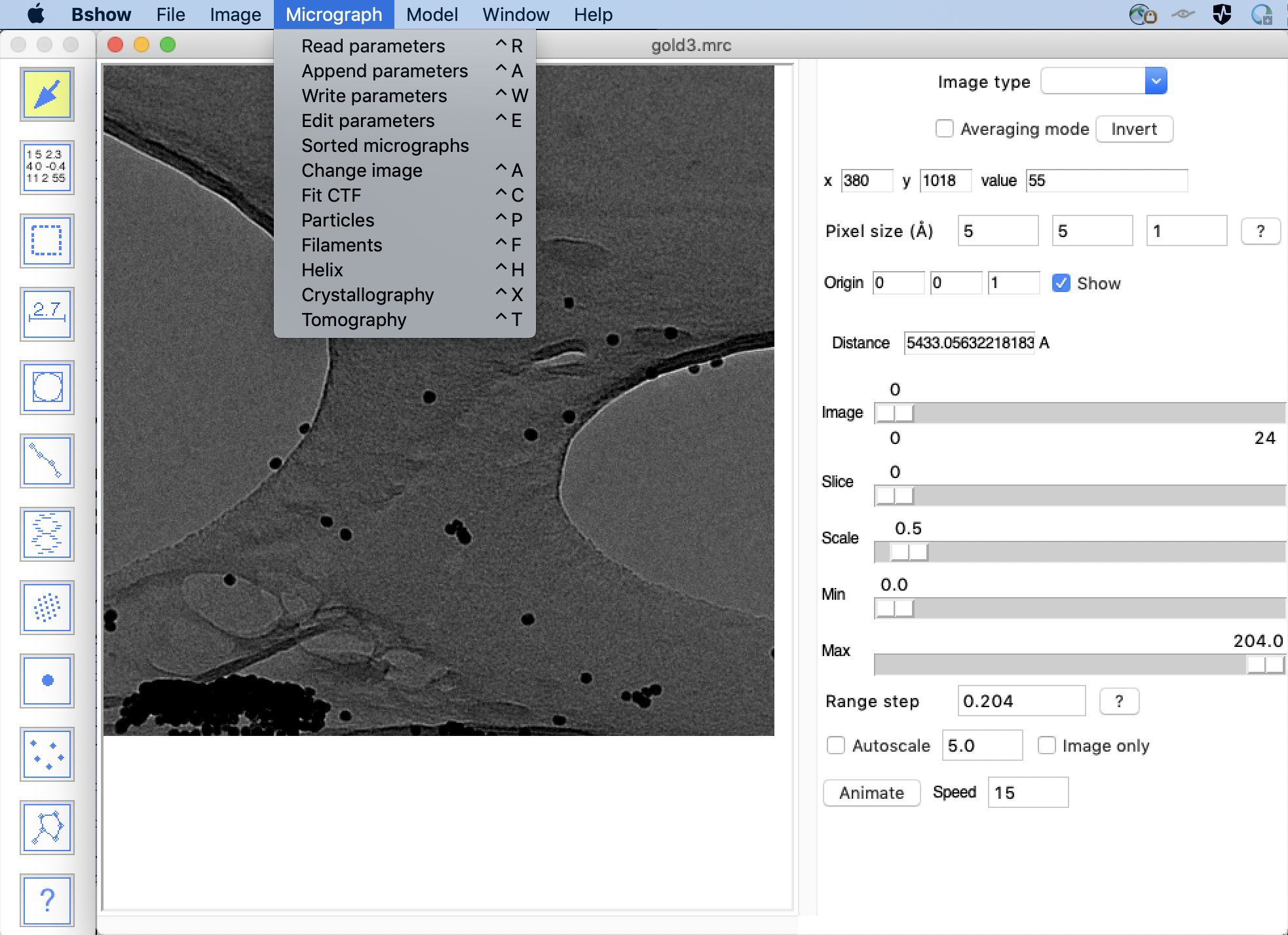
Open it in bshow to get the following display:

Tilt geometry convention

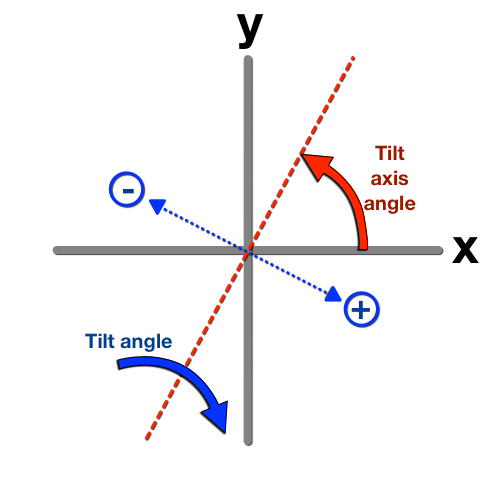
The tilt axis angle (red arrow) is defined as the angle relative to the x-axis and rotating anti-clockwise. The rotation around the tilt axis (red dashed line) is right-handed (blue arrow), so that the normal to the specimen plane rotates from negative to positive tilt angles. The normal to the specimen plane (dotted blue line) progresses from negative to positive tilt angles, from left to right (for a tilt axis close to the y-axis or 90˚) or top to bottom (for a tilt axis close to the x-axis or 0˚).

2. Setting the initial parameters

The initial parameters can be set up in a number of ways. The following sections detail three ways of doing it.

a. Using a SerialEM mdoc file

The program SerialEM is commonly used to acquire tilt series on electron microscopes. It produduces a text output file ending with the extension .mdoc. Bsoft programs can parse this file into its own internal parameter data base, setting up all the initial parameters. Note that the specification of the tilt axis angle in SerialEM is relative to the y-axis, while in Bsoft it is relative to the x-axis, giving a 90° difference.

Set up a new parameter file with btomo:

The -lamda parameter allows the estimation of the tomogram thickness, as described below. For fiducialless alignment, the btomaln program can read a .mdoc file directly and do the alignment without any other setup.

b. On the command line from an image file

Some of the initial parameters can be set up with btomo starting from a tilt series of images:

c. Using bshow

All of the initial parameters can be set up in bshow:

Set the following parameters:

• Enter the correct pixel size in the main window
• Select the menu item "Micrograph/Tomography" (see picture below)
• If the tilt series contain fiducial markers, enter the fiducial marker radius in pixels
• Enter the tilt axis angle
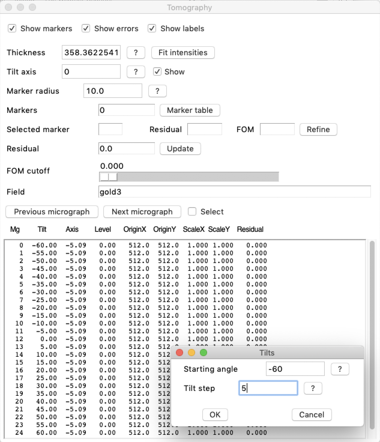
• Enter the tilt angles:
• Select the menu item "Tomography/Set tilt angles" and enter the the starting angle and the angular increment.
• or select the menu item "Tomography/Read rawtlt file" and read the angles from a *.rawtlt file

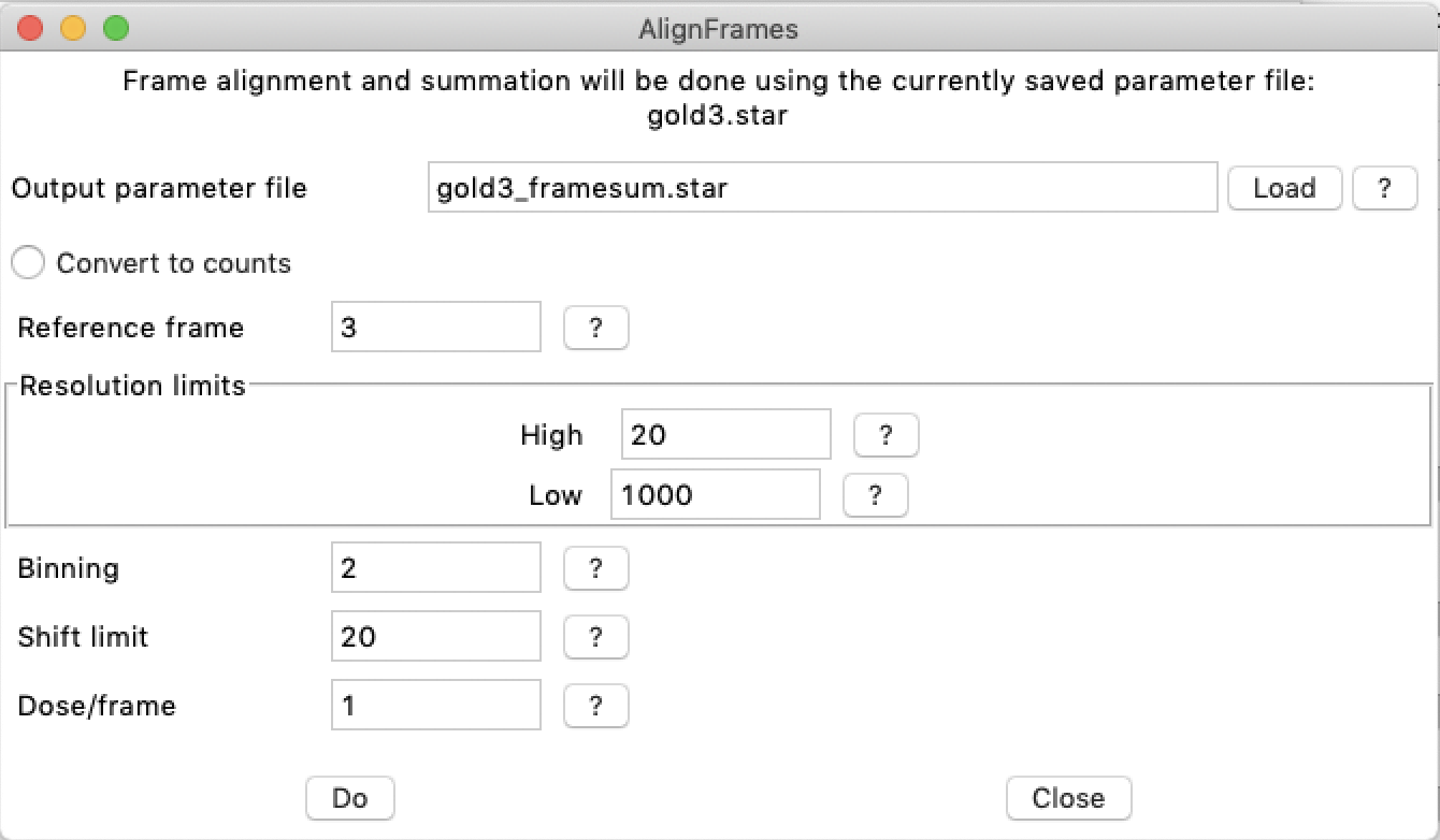
3. Aligning and summing frames

If each micrograph in the tilt series was acquired as multiple frames, they should be aligned and summed prior to any further operations.

3. Thickness estimation

The change in micrograph intensity can be used to estimate the thickness of the specimen, given a proportionality parameter, lambda (Λ). This parameter is often referred to as the "mean free path", but is not necessarily a true reflection of the mean distance between electron scattering events. Lambda is typically calibrated for a given microscope, acceleration voltage and imaging settings. The average intensity of a micrograph for a tilted specimen is given by:

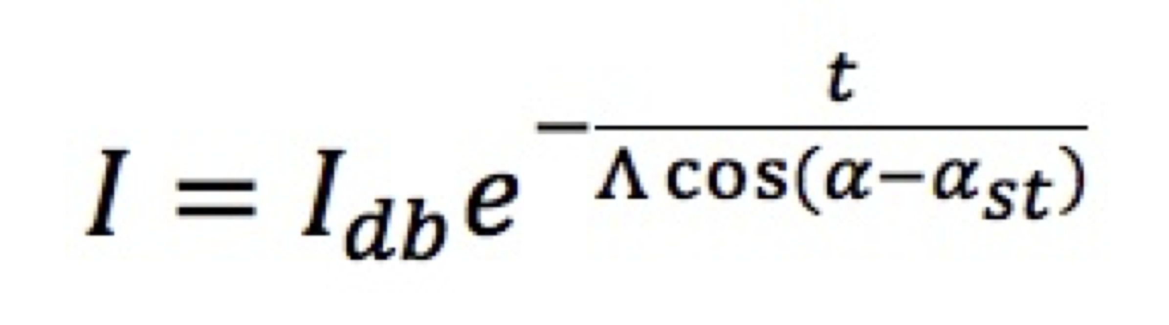
where I_db is the direct beam intensity, t is the average specimen thickness, α is the nominal tilt angle, and α_st is the specimen tilt angle for the nominal zero-degree micrograph.

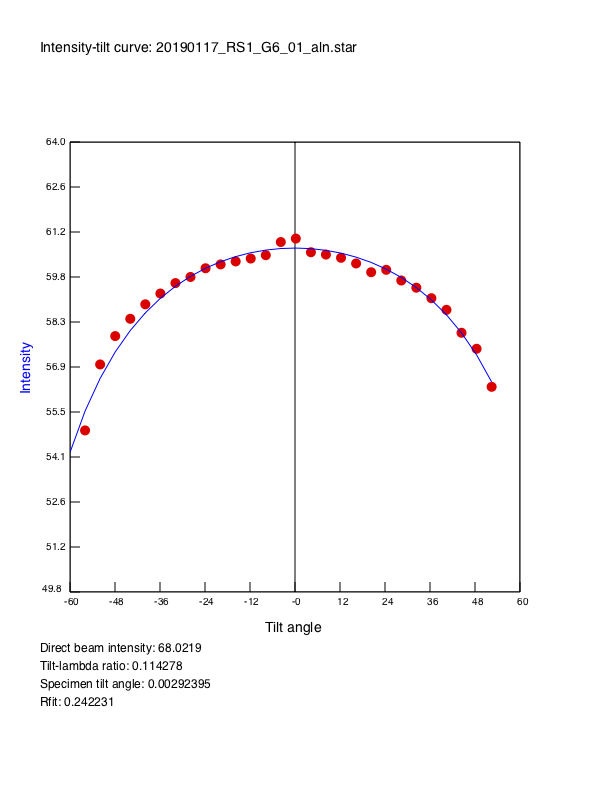
The parameter -lambda can be provided with several programs (btomo, btomaln) to estimate a specimen thickness. In the absence of a good value for it, the thickness-to-lambda ratio is calculated to allow for later calculation of the thickness once the appropriate value of lambda is established. With an appropriate value for lambda, the thickness can be estimated as follows:

An additional benefit of this analysis is that it gives an estimate of how much the specimen is tilted. The tilt angles are corrected to compensate for the specimen tilt. The -Postscript option generates a plot of the intensity change as well as the fit:

In the Tomography window in bshow, there is a "Thickness" entry. Click on the "Fit intensities" button to calculate the new specimen thickness. A dialog box will open with several options to do the fit. Set the lambda parameter to an appropriate value or click the button to estimate it from first principles. Check whether the result will be used to adjust the tilt angles. Finally, eneter a Postcript file name to generate a file with plot of intensities and fit. This file can be displayed with the "Open" button in an external display program (Preview on Mac OSX and ghostscript on Linux).

4. Normalization

In the traditional preparation of a tilt series, it was recommended to normalize the images to compensate for contrast variations. This is particularly important with film, where the dynamic range can vary considerably. With CCD cameras, it is less of an issue but still useful to render the contrast in images to a similar scale. With direct detectors, the more accurate representation of the signal makes it unnecessary to normalize the images. More importantly, the better reflection of actual counts means that the images are already properly weighted and should not be normalized. Note that normalization would also remove the information required for thickness estimation as described in the previous section.

If normalization is still desired, it can be done in several ways. The first is simply setting all the images to the same average and standard deviation:

The second is to fit the central part of the histogram of each micrograph to a Gaussian function, and rescale it to a given average and standard deviation:

Alternatively, the normalization can also be done using a previously generated parameter file: